Deep Structured Semantic Models
This is a post about Deep Structured Semantic Models (DSSM). DSSM is famous for its first application of deep structured models in the field of web search, where it was able to outperform traditional methods by a significant margin.
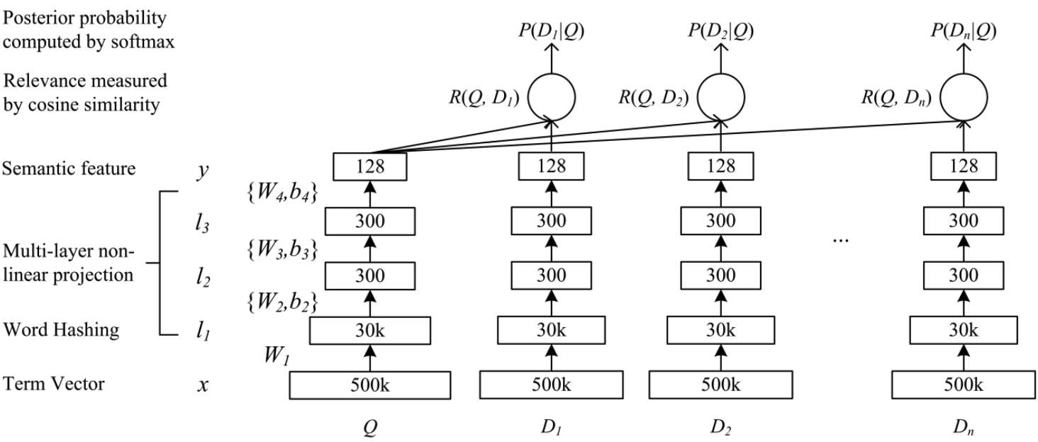
With pervasive large language models today, it may be unnecessary to understand how DSSM works. But from the view of application, algorithms/models that could achieve fairly good performance against small hardware cost is still a good choice. Here is the model architecture:

Suppose we have a query $Q$ and $n$ documents $D_i$ ($i=1,…,n$), we want to rank these documents according to their relevance to query Q.
The term vector $x$ actually is a one hot encoding of $Q$, each term within $Q$ could be represented as the count of its occurrence within $Q$. The same encoding also applied to document $D_i$. Or we should say term vector layer in DSSM model is just a one-hot encoded vector.
Then converting $Q$ to its word hashing. The original paper gives an example:
Suppose we have a term dictionay:
[good, quick, brown, fox]
Now we have a query $q_i$: good, then $q_i$ is encoded as: [1,0,0,0].
And next, we could split $q_i$ into following word hashs (3-grams):
#go, goo, #ood, od# (# is the special symbol indicating start or end of the query) and encode $q_i$ to 3-gram vector like this: [1,0,0,0,1,1,0,1] with following 3-gram dictionary:
[#go, all, but, can, goo,ood, you, od#]
Notice that position 1,5,6,8 are hit, so corresponding bits in the vector are set to 1.
The transition from term vector to word hashing could be seen as a fixed linear transformation as pointed by the paper so $W_1$ is not learnable parameter.
So after word hashing, we got a multi-hot vector $l_1$ with size $(30,000,)$.
Then from layer $2$ to $N-1$, we have the following transformation:
\[\begin{align*} l_i &= f(W_i l_{i-1} + b_i), i=2,...N-1 \\ y &= f(W_N l_{N-1} + b_N) \qquad (3) \end{align*}\]Where $tanh$ are the activation function:
\[f(x) = \frac{1 - e^{-2x}} {1 + e^{-2x} } \qquad (4)\]The semantic relevance between query $Q$ and a document $D$ is then measured as:
\[R(Q,D) = cosine(y_Q, y_D) = \frac{y_Q^T y_D}{\|y_Q \| \|y_D\|} \qquad (5)\]The DSSM model are learned on the click-through data, each example includes one positive document ($D^+$) and 4 negative documents (${ D_j^-; j=1,…4}$).
First, we compute the posterior probabilities of each document being relevant to a query:
\[P(D|Q) = \frac{exp(\gamma R(Q,D))}{\sum_{D' \in D} exp(\gamma R(Q, D'))} \qquad (6)\]In the training, the model parameters are estimated to maximize the likelihood of the clicked documents. The loss function is defined as:
\[L(\Lambda) = -log \prod_{Q,D^+} P(D^+ | Q) \qquad (7)\]where $\Lambda$ are the model parameters ${ W_i, b_i}$
Experiments(to be done)
Let’s first give an introduction to NDCG, from Wikipedia: NDCG is a measure used in Information Retrieval to evaluate ranking quality. It stands for Normalized Discounted Cumulative Gain, which is a normalized form of the DCG (Discounted Cumulative Gain). Lets give the definition of some terminologies:
- CG: is the sum of the graded relevance values ($rel_i$) in a search result list. The CG at a particular position $p$ is defined as:
One noticeble property is that CG is unaffected by changes in the ordering of search results (like for position of $1…(p-1)$)
- DCG: means discounted cumulative gain, the gains at position $i$ are discounted by a factor of $log_2(i+1)$:
An alternative definition of DCG is:
\[DCG_p = \sum_{i=1}^{p} \frac{2^{rel_i}-1}{log_2(i+1)}\]- IDCG: is the ideal discounted cumulative gain (Or we should say it is the ground truth value)
Now we could give the definition of NDCG:
\[nDCG_p = \frac{DCG_p}{IDCG_p}\]For the limitation of NDCG, you could check the wikipedia page of NDCG
References