Deep Neural Networks for YouTube Recommendations
The whole system is comprised of two neural networks, one for candidate generation and another for ranking.
Candidate Generation
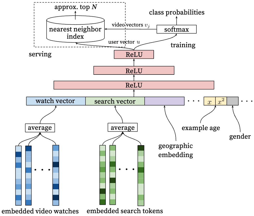
This problem is modeled as a classification problem, the target is to predict next video in a million-sized vedio pool based on user’s past behavior.
\[P(w_t = i | U, C) = \frac{e^{v_i u}}{\sum_{j \in V} e^{v_j u}}\]Where: $w_t$ is the vedio at time $t$; And $V$ is the video corpus;$U$ is the set of users; And $C$ is the context. $u \in \mathbb{R}^N$ respresents a high-dimensional user embedding
For the data used for training, a completed video is a positive example in the concext $C$ (we suppose that the previous watched, clicked vedios or other exposed videos are attributed as context)
Data sampling:
- Candidate sampling and correct this sampling via importance weighting.
Model architecture

Why use neural network as a genralization of matrix factorization?
The answer is with neural networks, arbitrary continuous and categorical features can be easily added into the model:
- Search history
- Tokens from both Unigram, bigram
- User demographic information
- Age, gender, location, and this is useful for new users.
- Watch history
- Simple binary and continuous features such as user’s gender, logged-in state and age are input directly into network as real value normalized to [0,1]
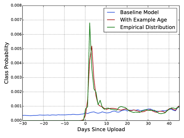
- “Example age” Feature, for video the lastest upload one is usually preferred by users. Without it, the model would usually recommend older videos which may not be what user wants. Here is a comparison with and without this feature for online watching:

Ranking model
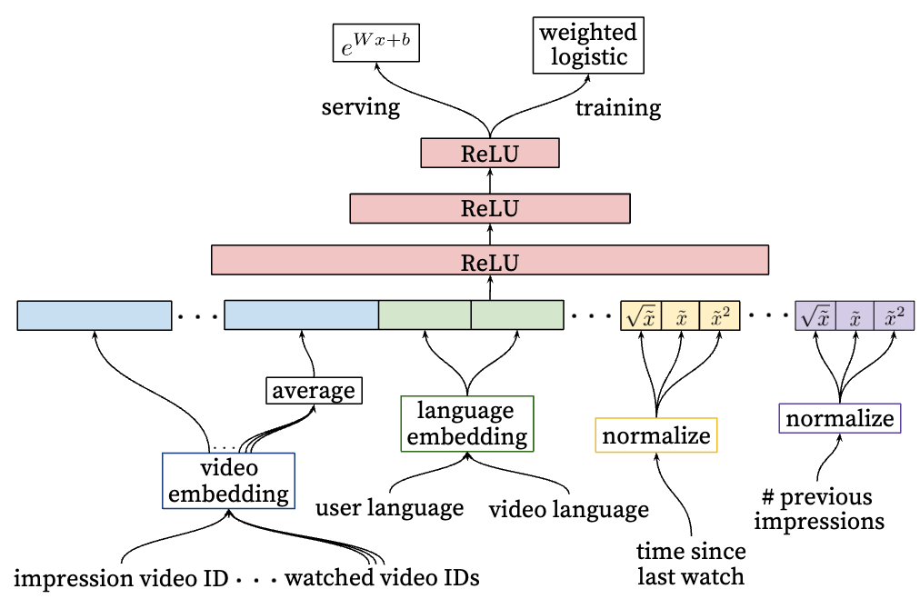
In ranking model, relationship between the user and video are more concerned. More features describing the user and the video relationship are added. The ranking model use the similar architecture with the recall model.
- Watch history
- last search query
- User’s previous interaction with the item and other similar items
- When was the user watch a video on this channel
- Propagate information from candidate generation into ranking in the form of feature. Which sources nominated this video candidate
Model Architecture

Positive and Negative examples
In ranking model, it use the weighted logistic regression for positive and negative examples, what does this “weighted” mean, here it means to design a specific value mappings so that to make these two classes values are weighted differently:
- Positive examples are annotated with the amount of time $t_{p_i}$ the user spent watching the video.
- Negative examples are annotated with unit watch time $t_{n_i}=1$. After applying the scoring function: $f(t) = e^t$, we could get:
After the training, the odds learned by the logistic regression are: $\frac{\sum T_i}{N-k}$, where $N$ is the number of training examples, $k$ is the number of positive impressions. Where $P$ is the click probability, and it is small; $T_i$ is the watch time of the $i$ th impression. And we should have:
\[\frac{\sum T_i}{N -k} \approx E[T](1 + P) \approx E[T]\]Embedding Categorical Features (Important)
- Unique IDs: to mapping these unique IDs to dense representations, we create embedding with its dimension proportional to the logrithm of the number of unique IDs
- Very large cardinality ID space (like video IDs or search query terms) are truncated by including the top $N$ most popular ones (measured by their click frequency).
- Out of vocabulary values are just mapped to zero embeddings.
- Categorical feature in the same space share the underlying embeddings.
- Like video ID, there are video ID of impression, last video ID watched by the user. Dispite shared embedding, but each feature is fed separately into the network. So that layers above could learn specicial representation of each feature. (most of the ID taken embedding dimension of 32)
Normalizing Continuous Features
- The author suggests to do value normalization for continuous features, scalling them, so that to make them distributed equally in range $[0,1)$
- A continuous feature $x$ with distribution $f$ is transformed to $\tilde x$ by scaling the values such that the feature is equally distributed in $[0, 1)$ using the cumulative distribution, $\tilde x = \int_{-\infty}^x df$
- Also powers based values are introduced, like $\tilde x^2$ and $\sqrt{\tilde x}$
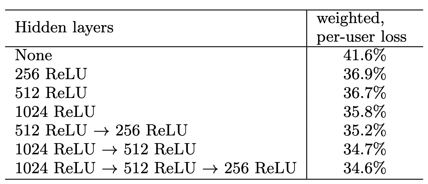
Best ranking model architeccure
 As we can see the last row of the table.